Lộc Lương

This was primarily a learning project for me, as I wanted to gain a solid understanding of deep learning algorithms. I ended up deciding to apply some popular neural network architectures, including Convolutional Neural Networks (CNNs) and Long Short-Term Memory networks (LSTMs), within a Generative Adversarial Network (GAN) framework. The goal is to predict stream flow using observed data from the Daymet dataset.

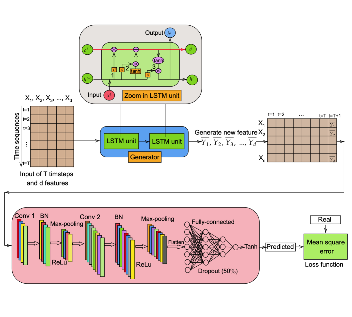
In this exploration of GAN architecture, I used a Long Short-Term Memory (LSTM) network as the generator, and a Convolutional Neural Network (CNN) as the discriminator. The LSTM generates new features, which are then combined with the existing training data and fed into the CNN discriminator to predict the stream flow. A mean squared error (MSE) loss function is used to minimize the discrepancy between the real and predicted values. Both the LSTM and CNN models are trained simultaneously on the training dataset, evaluated on the validation dataset, and tested to assess their generalization capability.

Model

Originally, GAN was proposed by Goodfellow et al. in 2014. The model is trained to learn the statistical patterns of input data, enabling it to generate outputs that resemble the original data. GANs have been widely applied in image generation, video prediction, and speech synthesis. The architecture consists of two fundamental components: a generator network and a discriminator network.

In this note, I slightly modified the GAN architecture to address the regression task of predicting stream flow. Figure below shows the development of the GAN model in this work, where the generator is implemented using a Long Short-Term Memory (LSTM) network and the discriminator is constructed using a Convolutional Neural Network (CNN).

The input data is made up of $T$ timesteps and $d$ features. The format of input data is as follows:

$$ X = [X_1, X_2, X_3, \dots, X_d] $$

where each column in input $X$ is a sequence of $T$ timesteps.

$$ X_i = \begin{bmatrix} X^1_i, X^2_i, X^3_i, \dots, X^T_i \end{bmatrix}^T, \quad \forall i = \overline{1 \dots d} $$

The input $X$ is fed into the LSTM (generator) network which consists of two LSTM units inside. As depicted in figure above, when we zoom in on the LSTM unit, there are several gates wherein the input data, previous hidden and cell state will pass through. To give better a intuitive view of LSTM, firstly, we define the parameters of the LSTM network as follows:

$$ W = \begin{bmatrix} W_f \ W_i \ W_c \ W_o \end{bmatrix}, \quad U = \begin{bmatrix} U_f \ U_i \ U_c \ U_o \end{bmatrix}, \quad b = \begin{bmatrix} b_f \ b_i \ b_c \ b_o \end{bmatrix} $$

where $W$ and $U$ are weight matrices and $b$ is bias vector; and $f$, $i$, $o$, $c$ indicate the forget gate, update gate, output gate, and cell state, respectively. The ability of LSTM to memory information that passes through the network comes from the cell state which is the red horizontal line running through the LSTM unit. At time step $t$, then input $X^{t}$ and the previous hidden state $h^{t-1}$ will pass through the forget gate (denote as 2).

$$ f_t = \sigma(W_f x_t + U_f h_{t-1} + b_f) $$

The second gate is the update gate which retains the information from the previous step to the cell state. There are two layers in this process: a sigmoid layer that decides the updated values and a tanh layer that creates new values. The output from those calculations will be added together with the output from forget gate through the element-wise multiplication operation $(\otimes)$ into the cell state (denote as 2).

$$ i_t = \sigma(W_i x_t + U_i h_{t-1} + b_i) $$

$$ \tilde{c}_t = \tanh(W_c x_t + U_c h_{t-1} + b_c) $$

$$ c_t = f_t \otimes c_{t-1} + i_t \otimes \tilde{c}_t $$

Finally, the output gate (denotes as 3) will control the output values from the LSTM unit. The mathematical expression is as follows:

$$ o_t = \sigma(W_o x_t + U_o h_{t-1} + b_o) $$

$$ h_t = o_t \otimes \sigma(c_t) $$

The output from the LSTM generator is transformed to the length of the input sequence, then reshaped and concatenated with the original input sequence to obtain a new input sequence that will be fed to the CNN discriminator. In the actual design architecture, there are two fully connected layers and a tanh activation layer at the end of the LSTM network:

$$ Y = \begin{bmatrix} \bar{Y}_1, \bar{Y}_2, \bar{Y}_3, \dots, \bar{Y}_d \end{bmatrix} $$

The CNN discriminator consists of two one-dimensional (1D) convolution layers, two batch normalization (BN) layers followed by two ReLU activation layers, two max-pooling layers, and two fully connected layers at the end. The first convolutional layer (Conv 1) receives the information from the LSTM generator and input sequences, then followed by a batch normalization layer and ReLU activation layer, and connected with the second convolutional layer (Conv 2) via a max-pooling layer. In accordance with the previous design, the second convolutional layers (Conv 2) are also followed by the batch normalization, the ReLU activation, and the max-pooling layers. Next, a flatten layer will be employed to convert the data into a one-dimensional array which is the input for the next two fully connected layers. Two dropout layers with a fifty percent probability of randomly dropping the units are also added to the networks to prevent the model from overfitting problem. Finally, the output from the whole GAN model is calculated through a tanh activation function wherein the output lies on the range from -1 to 1.

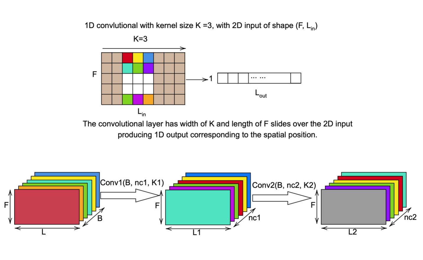
The input for the CNN discriminator has the shape of $(B, F, L )$, where $B$ is the batch size, $L$ is the sequence length (lag time or look back data), and $F$ is the number of features. Noting that the sequence length of CNN is now transposed to have more than one-time step compared to input length for LSTM.

On the advantages of this design of GAN, the batch norm layer help to train the networks faster and more stable since the output from previous layers is normalized and scaled into standard distribution, while the ReLU non-linear activation function help to deal with the vanishing gradient problem and less computational expensive than other activations such as tanh or sigmoid. As previously mentioned, dropout help to prevent the overfitting problem, and the max-pooling layers help to reduce the number of parameters, hence, improve the performance and avoid the overlearning issue.

It is worth noting that the loss function used in this study was mean square error which is different from the original proposed GAN model in the literature since this is a regression problem. By minimizing the discrepancy between the actual and predicted values through the loss function, the GAN model can learn from the historical data to capture the trend and be able to predict future performance. Finally, both generator and discriminator are trained simultaneously and iteratively. $$ \text{MSE} = \frac{1}{N} \sum_{i=1}^{N} \left( \hat{y}_i - y_i \right)^2 $$